Unsupervised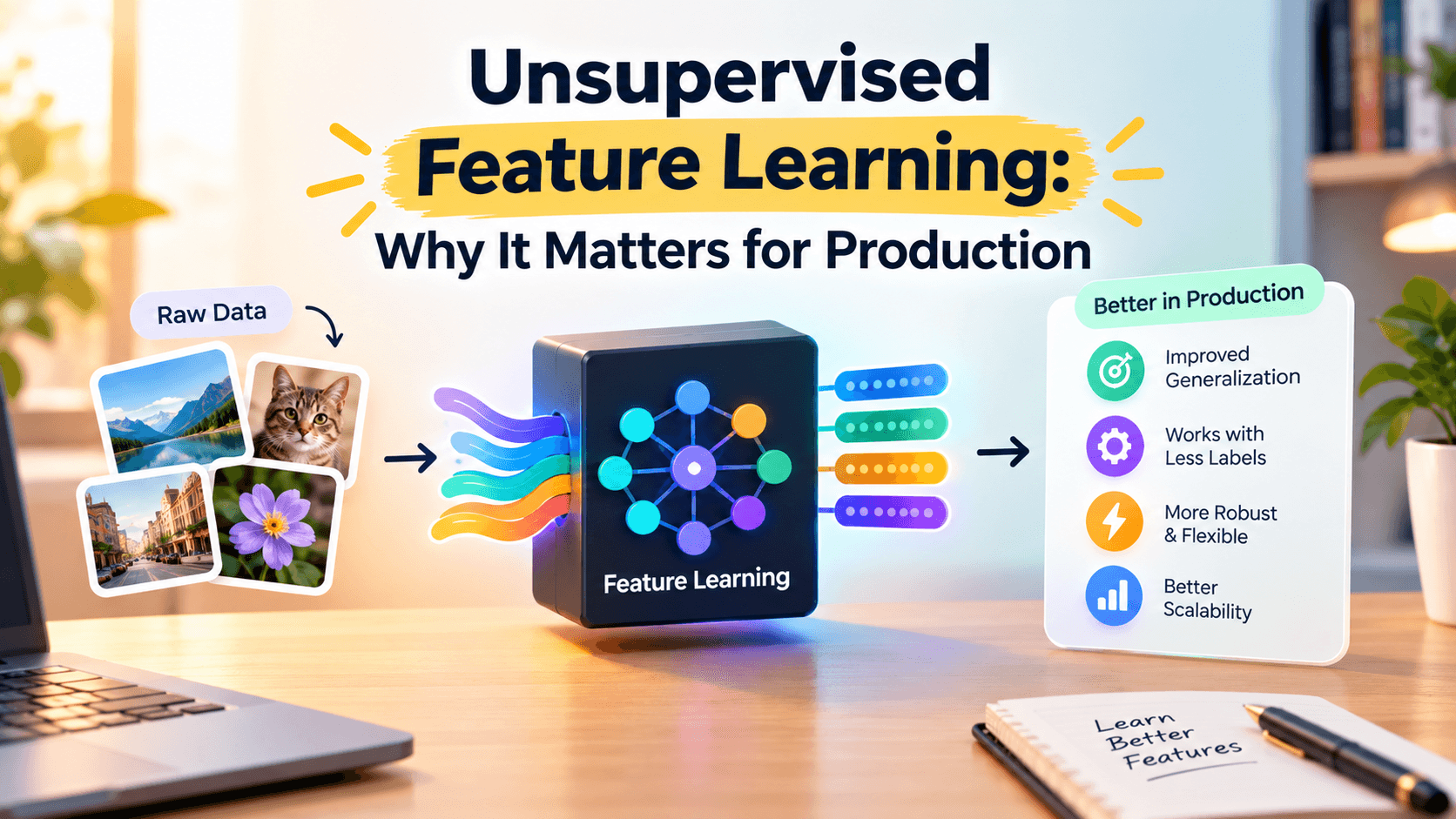 Feature Learning: Why It Matters for Production

In late 2024 While consultinging with a mid-stage healthcare startup that was trying to detect early-warning signs of patient deterioration from a continuous stream of vital signs. They had a labeled dataset of about 8,000 confirmed deterioration events and tens of millions of unlabeled vital-sign windows. Their initial instinct was to train a supervised model on the 8,000 events — and the model was bad, because 8,000 events weren't enough to learn the rich temporal patterns hidden in 6-lead ECG, SpO₂, respiration, and blood pressure signals. The breakthrough came when one of their engineers read a paper on contrastive predictive coding and proposed pre-training an encoder on the unlabeled windows first. Six weeks later they had a model that beat every supervised baseline they'd built, and they did it without collecting a single new label. That story is why This article article.

Why This Matters

Production machine learning in 2026 is dominated by an uncomfortable truth: labeled data is expensive, slow, and often impossible to obtain at scale. Medical imaging requires expert radiologist hours. Manufacturing defect detection requires domain experts to manually tag thousands of parts. Fraud labels require chargeback resolution that may take 90 days. Meanwhile, unlabeled data is often streaming in continuously — every user interaction, every sensor reading, every log line.

The traditional supervised learning paradigm pretends this asymmetry doesn't exist. The unsupervised feature learning paradigm embraces it. The idea is straightforward: train a model to learn useful representations from unlabeled data, then either fine-tune those representations on a smaller labeled set or use them as direct inputs to a downstream classifier or regressor.

The production impact is enormous. Self-supervised and unsupervised pre-training has become a default stage in modern computer vision pipelines (SimCLR, DINO, MAE), in NLP (BERT, RoBERTa, the entire family of transformer pre-training approaches), in time-series (TS2Vec, contrastive predictive coding), and in tabular ML (TabNet's pretraining stage, contrastive tabular learning). If you're building a production ML system in 2026 and you're not at least considering unsupervised pre-training as part of your pipeline, you're leaving substantial accuracy on the table.

The numbers are dramatic. The healthcare startup It mentioneds improved their AUC from 0.78 (supervised only) to 0.91 (self-supervised pre-training plus fine-tuning on the same labeled set). The unlabeled pretraining stage added a meaningful performance ceiling that supervised-only training simply couldn't reach with their labeled budget.

There's a deeper reason this matters beyond raw accuracy: unsupervised features tend to be more robust to distribution shift. When your model has learned representations that capture the underlying structure of the data rather than memorizing labeled patterns, it generalizes better to new populations, new sites, new time periods. For production systems that have to survive concept drift, this robustness matters as much as accuracy.

The Core Idea

Unsupervised feature learning is a broad category that includes several distinct approaches. They all share the goal of learning a mapping f: X → Z from raw inputs to a representation space, where Z is "useful" — useful being defined loosely as making downstream tasks easier. The differences are in how "useful" is defined operationally.

The classical approach is autoencoders. Train a neural network to compress the input into a low-dimensional bottleneck and then reconstruct it. The bottleneck activations are the learned features. The intuition is that to reconstruct the input well, the network must capture the most informative patterns. Variational autoencoders (VAEs) add a probabilistic structure: the bottleneck is constrained to follow a Gaussian prior, which gives you a smooth, generative latent space you can sample from.

Autoencoders are old-school but they're not obsolete. For tabular data, especially in regulated industries where you need interpretability, a well-tuned autoencoder with a low-dimensional bottleneck produces features that are surprisingly competitive with self-supervised methods. They also have a useful failure mode: reconstruction error is itself an anomaly score. If you train an autoencoder on normal data, samples with high reconstruction error are likely anomalous.

The second major approach is contrastive learning. The idea is to train a model to identify which samples are "similar" and which are "different." In SimCLR, you take an input image, generate two augmented views of it, and train the network to produce embeddings such that the two views are close together while being far from all other images in the batch. The augmentations (random crops, color jitter, blur) define what "similar" means operationally. The network learns features invariant to those augmentations.

Contrastive learning exploded in computer vision from 2020 onward. The pattern has since been ported to time-series (TS2Vec uses hierarchical contrastive learning across timestamps), to graph data (graph contrastive learning), to audio (wav2vec 2.0), and to tabular data (contrastive tabular learning, where you generate augmented "views" by mixing features).

The third approach is masked reconstruction. You take an input, mask out some fraction of it (random patches for images, random tokens for text, random time windows for time-series), and train the network to predict the missing parts. BERT is the canonical example for text. MAE (Masked Autoencoders) extended the idea to images and showed that simply reconstructing masked patches produces remarkably general features.

Masked reconstruction has a different inductive bias than contrastive learning. Contrastive methods tend to learn features that emphasize discriminative structure — what makes samples different. Masked reconstruction learns features that emphasize generative structure — what the data looks like as a whole. In practice they often produce complementary features. Some recent systems use both in a multi-task pretraining stage.

A fourth approach worth mentioning is distillation-based self-supervision, popularized by DINO and DINOv2 in vision. Train a student network to match the output of a teacher network on different augmented views of the same image. The teacher is updated as an exponential moving average of the student. This produces features with surprisingly strong transfer performance and is what's behind many of the foundation models released in 2024 and 2025.

For tabular production ML specifically, the practical options are more limited. TabNet has a self-supervised pretraining stage where you mask features and predict them. SAINT does the same with a transformer architecture. There's also a body of work on contrastive learning for tabular data that uses mixup-style augmentations. The improvements over supervised-only training are real but smaller than the gains you see in vision or NLP — typically 2-5% AUC on downstream tasks.

A Concrete Example

The following walks through a realistic tabular ML pipeline using a denoising autoencoder for pretraining. We'll use the UCI Adult dataset as a stand-in for any moderately-sized tabular classification problem. The setup: you have a labeled training set and a much larger unlabeled set you want to leverage. The pattern generalizes to fraud detection, churn prediction, and most production tabular tasks.

import numpy as np
import pandas as pd
import torch
import torch.nn as nn
from torch.utils.data import DataLoader, TensorDataset
from sklearn.preprocessing import StandardScaler, OneHotEncoder
from sklearn.compose import ColumnTransformer
from sklearn.model_selection import train_test_split
from sklearn.linear_model import LogisticRegression
from sklearn.metrics import roc_auc_score

# Load the Adult dataset as a generic tabular example
url = "https://archive.ics.uci.edu/ml/machine-learning-databases/adult/adult.data"
columns = ["age", "workclass", "fnlwgt", "education", "education-num",
           "marital-status", "occupation", "relationship", "race", "sex",
           "capital-gain", "capital-loss", "hours-per-week",
           "native-country", "income"]
df = pd.read_csv(url, header=None, names=columns, na_values=" ?",
                 skipinitialspace=True)
df = df.dropna().reset_index(drop=True)

y = (df["income"].str.strip() == ">50K").astype(int).values
X = df.drop(columns=["income"])

# Identify categorical and numeric columns
cat_cols = X.select_dtypes(include=["object"]).columns.tolist()
num_cols = X.select_dtypes(include=["int64", "float64"]).columns.tolist()

preprocessor = ColumnTransformer([
    ("num", StandardScaler(), num_cols),
    ("cat", OneHotEncoder(handle_unknown="ignore", sparse_output=False), cat_cols),
])
X_processed = preprocessor.fit_transform(X)
print(f"Processed feature dimension: {X_processed.shape[1]}")

X_train, X_test, y_train, y_test = train_test_split(
    X_processed, y, test_size=0.2, random_state=42, stratify=y,
)

# Pretend we have a much larger unlabeled pool. In real life, this would be
# data you couldn't label due to budget or time. Here we simulate by ignoring
# labels on a subset.
X_unlabeled_pool = X_processed[len(X_train):]
X_train_labeled = X_train[:1500]   # restrict labels to mimic real-world budget
y_train_labeled = y_train[:1500]

# --- Denoising Autoencoder Pretraining ---
# We mask random feature columns and ask the network to reconstruct them.
# The encoder learns features robust to missingness — a useful property
# for production data with intermittent nulls.

class DenoisingAutoencoder(nn.Module):
    def __init__(self, input_dim, hidden_dim=128, latent_dim=32):
        super().__init__()
        self.encoder = nn.Sequential(
            nn.Linear(input_dim, hidden_dim),
            nn.ReLU(),
            nn.BatchNorm1d(hidden_dim),
            nn.Linear(hidden_dim, latent_dim),
        )
        self.decoder = nn.Sequential(
            nn.Linear(latent_dim, hidden_dim),
            nn.ReLU(),
            nn.BatchNorm1d(hidden_dim),
            nn.Linear(hidden_dim, input_dim),
        )

    def forward(self, x, mask=None):
        if mask is None:
            mask = torch.bernoulli(torch.full_like(x, 0.85))  # keep 85% of features
        x_masked = x * mask / 0.85  # invert scaling to preserve magnitude
        z = self.encoder(x_masked)
        x_hat = self.decoder(z)
        return x_hat, z


input_dim = X_train.shape[1]
device = "cuda" if torch.cuda.is_available() else "cpu"
model = DenoisingAutoencoder(input_dim).to(device)
optimizer = torch.optim.AdamW(model.parameters(), lr=1e-3, weight_decay=1e-5)
criterion = nn.MSELoss()

unlabeled_loader = DataLoader(
    TensorDataset(torch.tensor(X_unlabeled_pool, dtype=torch.float32)),
    batch_size=256, shuffle=True,
)

# Pretraining loop — note we only use features, never labels.
for epoch in range(20):
    model.train()
    epoch_loss = 0
    for (x,) in unlabeled_loader:
        x = x.to(device)
        mask = torch.bernoulli(torch.full_like(x, 0.85))
        x_hat, _ = model(x, mask)
        loss = criterion(x_hat, x)
        optimizer.zero_grad()
        loss.backward()
        optimizer.step()
        epoch_loss += loss.item() * len(x)
    print(f"epoch {epoch+1:>2d}  pretrain MSE = {epoch_loss/len(X_unlabeled_pool):.4f}")

# --- Extract Features and Train a Classifier ---
# Freeze the encoder and use its latent outputs as features.
model.eval()
with torch.no_grad():
    Z_labeled = model.encoder(torch.tensor(X_train_labeled,
                                           dtype=torch.float32).to(device))
    Z_test = model.encoder(torch.tensor(X_test, dtype=torch.float32).to(device))

# Baseline: supervised logistic regression on raw features
clf_raw = LogisticRegression(max_iter=1000).fit(X_train_labeled, y_train_labeled)
auc_raw = roc_auc_score(y_test, clf_raw.predict_proba(X_test)[:, 1])

# Pretrained: logistic regression on the learned 32-dim representation
clf_pt = LogisticRegression(max_iter=1000).fit(Z_labeled.cpu().numpy(),
                                               y_train_labeled)
auc_pt = roc_auc_score(y_test, clf_pt.predict_proba(Z_test.cpu().numpy())[:, 1])

print(f"\nSupervised-only AUC:    {auc_raw:.3f}")
print(f"Pretrained features AUC: {auc_pt:.3f}")
print(f"Improvement:             {auc_pt - auc_raw:+.3f}")

The numbers will vary based on your random seed, but you should see the pretrained-features AUC meaningfully beat the supervised-only baseline. The encoder has learned to compress 100+ raw features into 32 dimensions that preserve the structure of the data, and that representation transfers well to the classification task even though the pretraining never saw a single label.

For deployment, you save both the encoder and the downstream classifier:

# Production inference path:
# 1) Preprocess incoming tabular features with the same ColumnTransformer
# 2) Pass through the encoder to get 32-dim embedding
# 3) Pass embedding through logistic regression to get probability
# 4) Apply business threshold and serve

# Save the pipeline
import joblib

torch.save(model.state_dict(), "denoising_ae.pt")
joblib.dump(clf_pt, "downstream_lr.joblib")
joblib.dump(preprocessor, "preprocessor.joblib")

# At inference time
def predict_proba(raw_input_df):
    X = preprocessor.transform(raw_input_df)
    Z = model.encoder(torch.tensor(X, dtype=torch.float32).to(device))
    return clf_pt.predict_proba(Z.detach().cpu().numpy())[:, 1]

That four-step inference path is what production unsupervised feature learning actually looks like. The encoder is a feature extractor; the downstream classifier is trained on top; both get versioned and deployed together.

Common Pitfalls

Pretraining on data that doesn't match deployment distribution. This is the number-one failure mode in production. If you pretrain on data from one hospital but deploy at another, the learned features won't transfer. Always pretrain on data that reflects the deployment context — and if you must mix sources, weight by deployment frequency.
Forgetting that pretraining has its own hyperparameters. Autoencoder hidden dimension, latent dimension, learning rate, mask ratio, contrastive temperature — these all matter. Bad choices can produce features worse than raw input. Always evaluate the pretrained features on a downstream task using cross-validation before shipping them.
Treating unsupervised pretraining as a substitute for labels. It's not. The features are useful, but you still need a labeled validation set to evaluate downstream quality and a labeled test set to confirm the system actually works. Unsupervised pretraining makes your labeled data more efficient, it doesn't eliminate the need for labels.
Skipping data quality checks on the unlabeled pool. Unsupervised pretraining amplifies whatever's in the unlabeled data — including biases, distribution shifts, and quality issues. If your unlabeled pool is dominated by a subpopulation that doesn't appear at inference time, the encoder will overfit to that subpopulation's idiosyncrasies. Audit the unlabeled pool's distribution before pretraining.
Using the wrong pretraining objective for the downstream task. Contrastive features are great for classification. Masked reconstruction features are great for tasks where local structure matters. Autoencoder features are great when reconstruction error is itself a useful signal (anomaly detection). Pick the pretraining objective based on the downstream use case, not based on which paper was most cited recently.

When to Use This (And When Not To)

Use unsupervised feature learning whenever your labeled data is expensive relative to your unlabeled data. The classic case is medical imaging, where expert annotation is slow and unlabeled archives are huge. It's also valuable in fraud detection, where labels require chargeback resolution cycles measured in weeks. And it's become standard in time-series anomaly detection, where unlabeled streams are abundant and confirmed anomalies are rare.

Skip unsupervised pretraining when you have abundant labeled data. If you already have 100 million labeled examples, pretraining on unlabeled data is unlikely to help much. The marginal value of unsupervised pretraining decreases as labeled data grows. Compute the cost-benefit honestly.

Skip it when the unlabeled pool has wildly different distribution from deployment. Pretraining on the wrong distribution hurts more than helps. You can sometimes rescue this with domain adaptation techniques, but that's a separate engineering project.

Skip it for simple models. If your downstream task is well-served by a logistic regression on a small number of hand-crafted features, unsupervised pretraining is overkill. The benefit is mainly felt when the downstream model is a deep neural network that can use rich representations.

Wrapping Up

Unsupervised feature learning is one of the highest-leverage techniques available to production ML teams in 2026. It directly addresses the labeled data scarcity problem that limits most enterprise ML efforts, and it produces representations that generalize better to distribution shift than purely supervised models. Take any tabular or time-series pipeline you maintain, identify your largest pool of unlabeled data, and try pretraining a denoising autoencoder on it. Evaluate the resulting features on your existing labeled test set. The improvement you measure will tell you whether to invest further.